Kinematics and Visualization

Chapter description

In this chapter, we will first discuss the theory that makes a robot without a torsion axis change its direction of travel. Then you will be able to drive the rosbot using the keyboard or joystick and use tools such as plot_joggler and RViz, which allow for eye-pleasing data visualization.

You can run this tutorial on:

• ROSbot 2 PRO
• ROSbot 2R
• ROSbot 2R (Gazebo simulation)

Repository containing the final effect after doing all the ROS Tutorials you can find here

Robot control - theory

The purpose of forward kinematics in mobile robotics is to determine robot position and orientation based on wheels rotation measurements. To achieve that we'll create a robot kinematic model. ROSbot is a four wheeled mobile robot with separate drive for each wheel, but in order to simplify kinematic calculation we will treat it as two wheeled. Two virtual wheels (marked as W_L and W_R on the scheme) will have axes going through the robot geometric center. This way we can use a simpler kinematic model of differential wheeled robot. The name "differential" comes from the fact that a robot can change its direction by varying the relative rate of rotation of its wheels and does not require additional steering motion. Robot scheme is presented below:

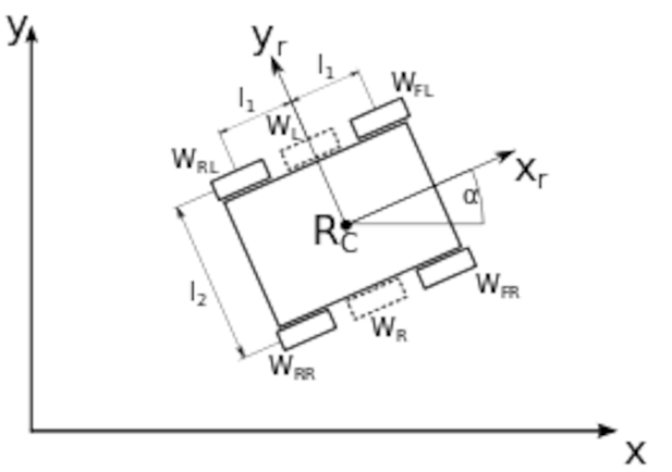
Description:

• R_c - robot geometric centre
• x_c - robot geometric centre x position
• y_c - robot geometric centre y position
• x_r - robot local x axis that determines front of the robot
• y_r - robot local y axis
• $α$ - robot angular position
• W_FL - front left wheel
• W_FR - front right wheel
• W_RL - rear left wheel
• W_RR - rear right wheel
• W_L - virtual left wheel
• W_R - virtual right wheel
• l₁ - distance between robot center and front/rear wheels
• l₂ - distance between robot left and right wheels

Our mobile robot has constraints. It can only move in x-y plane and it has 3 DOF (degrees of freedom). However not all of DOFs are controllable which means the robot cannot move in every direction of its local axes (e.g. it cannot move sideways). Such drive system is called non-holonomic. When amount of controllable DOFs is equal to total DOFs then a robot can be called holonomic. To achieve that some mobile robots are built using Omni or Mecanum wheels and thanks to vectoring movement they can change position without changing their heading (orientation).

Forward Kinematics task

The robot position is determined by a tuple (x_c, y_c, $α$). The forward kinematic task is to find new robot position (x_c, y_c, $α$)' after time $dt$ for given control parameters:

In our case the angular position $\phi$ and the angular speed $\omega$ of each virtual wheel will be an average of its real counterparts:

$$\begin{align*} \phi{W_L} &= \frac{\phi{W_{FL}}+\phi{W_{RL}}} 2 \qquad \phi{W_R} = \frac{\phi{W_{FR}}+\phi{W_{RR}}} 2 \\ \omega{W_L} &= \frac{\omega{W_{FL}}+\omega{W_{RL}}} 2 \qquad \omega{W_R} = \frac{\omega{W_{FR}}+\omega{W_{RR}}} 2 \end{align*}$$

The linear velocity of any virtual circle can be calculated by multiplying the angular velocity times the radius of the circle:

$$v_L = \omega{W_{L}}\cdot{r} \qquad v_R = \omega{W_{R}}\cdot{r}$$

where,

• v_L - linear speed of left virtual wheel
• v_R - linear speed of right virtual wheel
• r - the wheel radius.

We can determine robot angular position and speed with:

$$\alpha=(\phi{W_R}-\phi{W_L})\cdot\frac r l_2$$ $$\dot\alpha=\frac {d\alpha} {dt}$$

Then robot speed x and y component:

$$\dot{x}_c=(v_L+\dot\alpha\cdot\frac r l_2)\cos{\alpha}$$ $$\dot{y}_c=(v_L+\dot\alpha\cdot\frac r l_2)\sin{\alpha}$$

To get position:

$$x_c=\int^t_0\dot{x}_cdt \qquad y_c=\int^t_0\dot{y}_cdt$$

We assume starting position as (0,0).

Above equations are implemented in your ROSbot and can be found here.

Robot control - practice

Most common way to send movement commands to the robot is with use of geometry_msgs/Twist message type. Then the motor driver node should use data stored in them to control the motor. The geometry_msgs/Twist message express velocity in free space and consists of two fields:

• Vector3 linear - represents linear part of velocity [m/s]
• Vector3 angular - represents angular part of velocity [rad/s]

You will control ROSbot in the x-y plane by sending appropriate values to /cmd_vel. Namely, value x manipulating the component of linear speed vector and the z component of angular speed vector.

Robot speed control

Below is a simple example of posting a speed message using the keyboard. The geometry_msgs/Twist message is used for this purpose. The node that publishes it is called teleop_twist_keyboard from the package teleop_twist_keyboard. Alternatively you can use the joystick to control the robot, then you will need a joy_node from the joy package and a teleop_node from the teleop_twist_joy package. To run the node and control the robot using the keyboard, enter the following command.

ROSbot

husarion@husarion:~$

docker compose up -d rosbot ros-master
rosrun teleop_twist_keyboard teleop_twist_keyboard.py

Gazebo simulator

You need to first start simulator.

user@mylaptop:~$

roslaunch rosbot_bringup rosbot_tutorial.launch

Then in the new terminal run teleop_twist_keyboard.

user@mylaptop:~$

rosrun teleop_twist_keyboard teleop_twist_keyboard.py

Now you can control your robot with keyboard with following functions for buttons:

• ’i’ - move forward
• ’,’ - move backward
• ’j’ - turn left
• ’l’ - turn right
• ’k’ - stop
• ’q’ - increase speed
• ’z’ - decrease speed

Checking state of robot

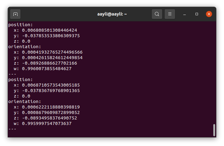
Below is an example that allows you to read the current position in the terminal. To do this, open a new term and do:

husarion@husarion:~$

rostopic echo /odom

After executing the above command, information about the current location should appear in the terminal, it looks like this.

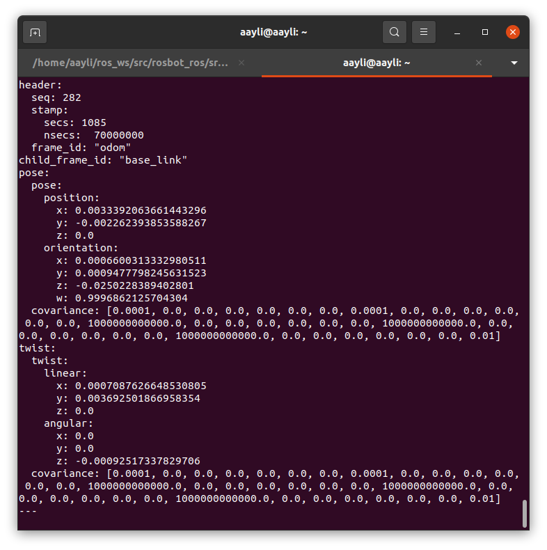
The presented format is related to the type of message used to determine the state of the robot, a message of the nav_msgs/Odometry type containing information about speeds (twist) and positions (pose) is used. If you would like to get data only for specific fields, you can add the names of these fields to the name of the message. Example:

husarion@husarion:~$

rostopic echo /odom/pose/pose

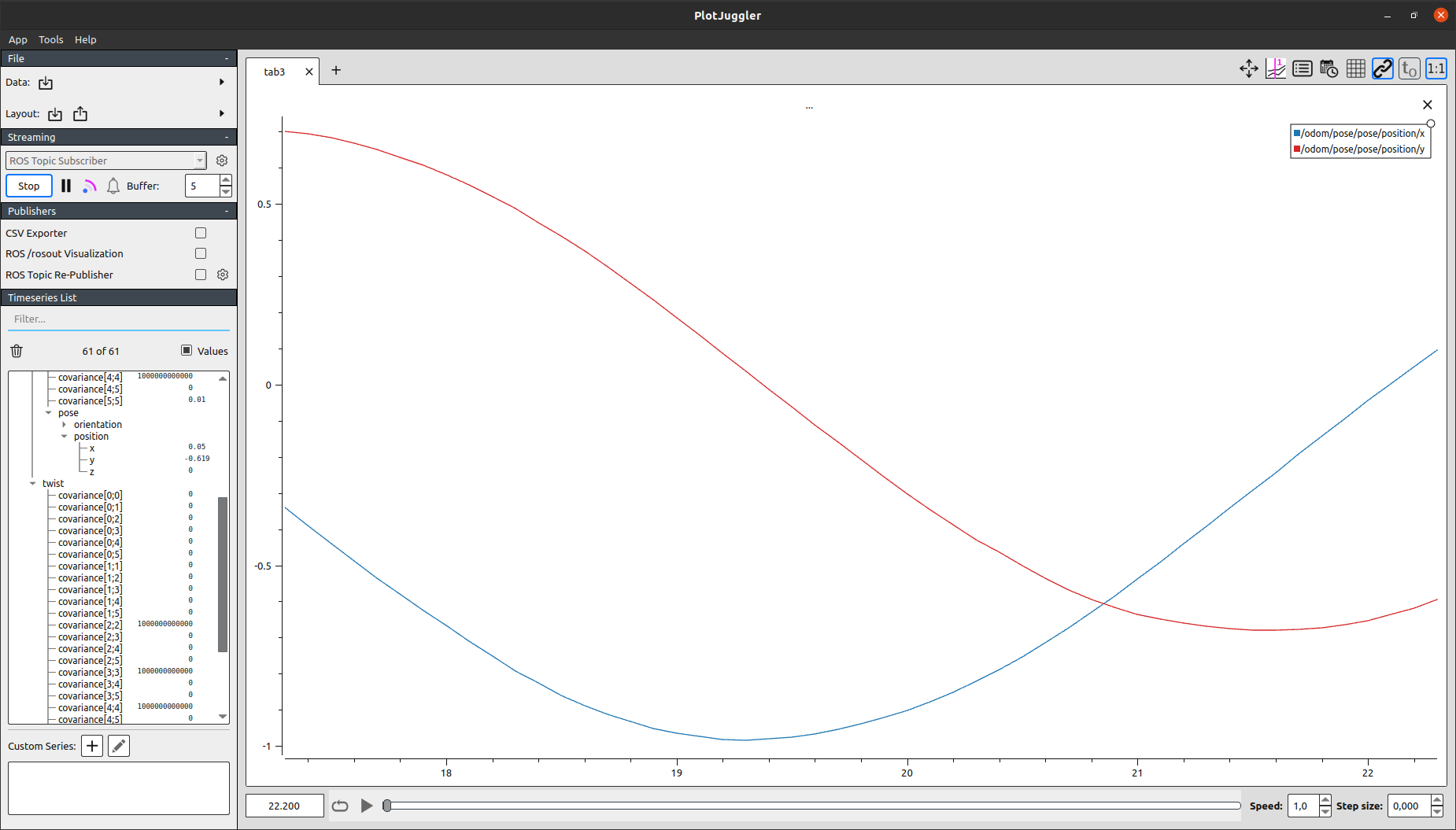
Data visualization with PlotJuggler

In this section you will learn how to visualize data from ros topics using PlotJuggler. It is a simple tool that allows you to plot logged data, in particular timeseries. You can learn more about the tool on its official webpage.

Install additional package

To install additional package you can type:

husarion@husarion:~$

sudo apt-get install ros-$ROS_DISTRO-NAME-OF-PACKAGE

For PlotJuggler use:

husarion@husarion:~$

sudo apt-get install ros-$ROS_DISTRO-plotjuggler-ros

And run it:

husarion@husarion:~$

rosrun plotjuggler plotjuggler

From menu bar select Streaming > Start: ROS Topic Subscriber. In pop-up menu that will appear choose /odom from available topic names and press ok. To visualize data drag interested field from Timeseries List and drop it on the figure area. This way you can comfortably observe multiple values from odometry data during robot motion.

Data visualization with RViz

RViz is tool which allows visualization of robot position, traveled path, planned trajectory, sensor state or obstacles surrounding robot.

To run it type in terminal:

husarion@husarion:~$

rviz

New window will appear:

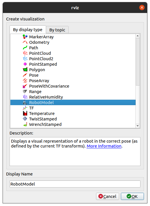
By default you will see only empty space, to add any other object push Add. In new window, there are two tabs By display type and By topic. First one is for manual selection from all possible objects, second one contains only currently published topics. Find RobotModel in By display type tab and press OK.

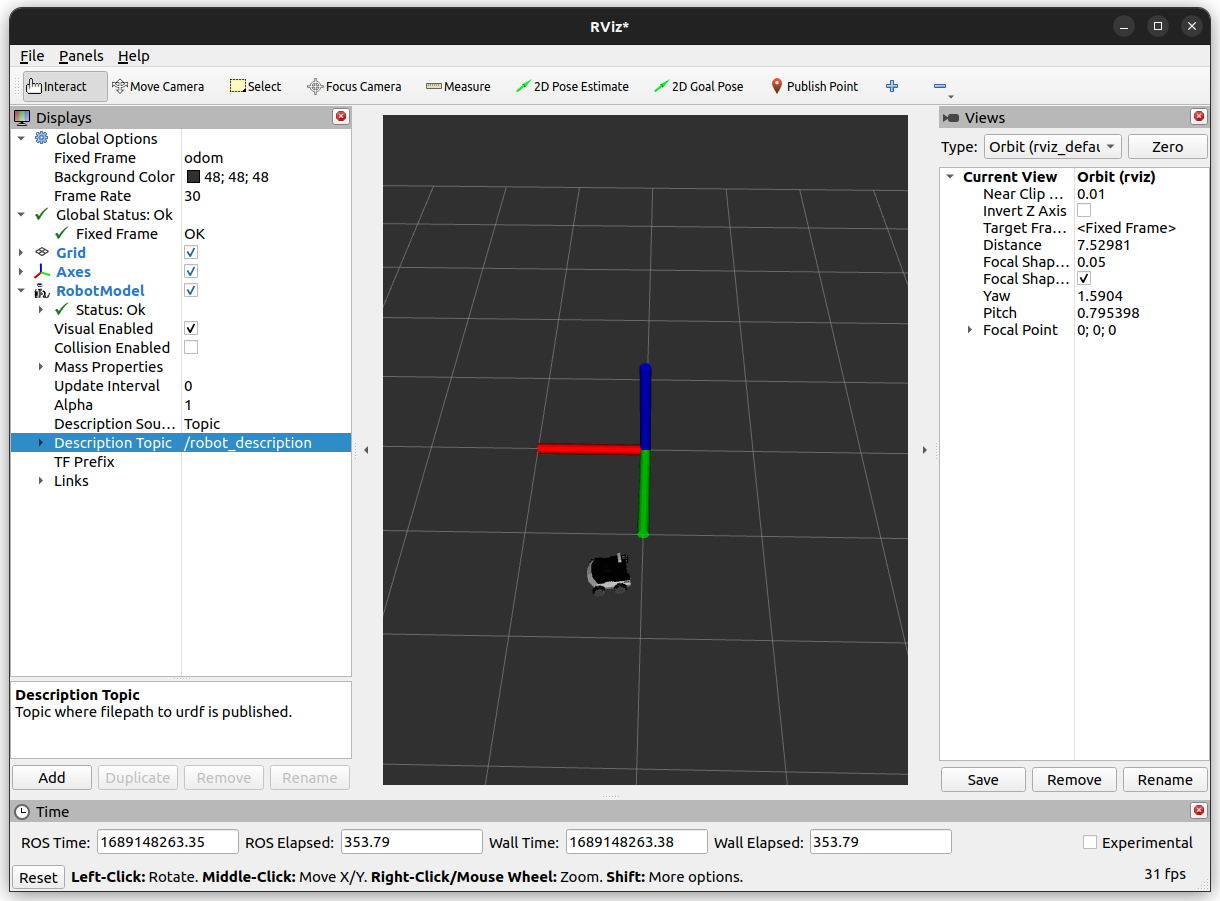
Then, in new left panel in RobotModel, find Description Topic and select /robot_description. You should see white object on the middle of space. This is because there is no defined transformation between the robot's position and the defined map reference system. To fix this, select the odom frame in the Fixed Frame field.

Now ROSbot should be visible. Let's add a global frame of reference. To do this, press again Add and select Axes.

The last thing will be added odometry msg. Click Add->By topic->/odom. Information about covariance isn't necessary so we disable it Odometry->Covariance.

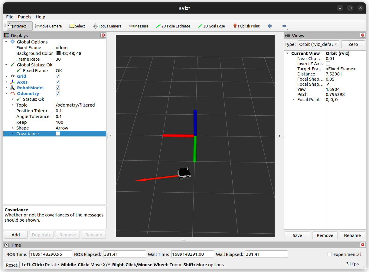
After this is done, you should see an arrow representing position and orientation of your robot. You will also see a representation of coordinate frames bounded with robot starting position and robot base. Move your robot and observe as the arrow changes its position.

Now lest save this configuration. Go to File->Save Config As and save it as rosbot.rviz in the new folder ~/ros_ws/src/tutorial_pkg/rviz.

Now RViz can be launched with argument pointing to file .rviz. To do this use:

husarion@husarion:~$

rviz -d ~/ros_ws/src/tutorial_pkg/rviz/rosbot.rviz

or add this line to launch file

<node name="rviz" pkg="rviz" type="rviz" args="-d $(find tutorial_pkg)/rviz/rosbot.rviz"/>

Task 1

Try adding the camera node to your launch file and visualize image in your current RViz configuration (in simulation camera node is already started - you don't need to modify launch file).

Summary

After completing this tutorial you should understand the math that enables the robot to move. You be able to control your ROSbot, change desired velocity and have better knowledge of new types of message like geometry_msgs/Twist, geometry_msgs/Pose and nav_msgs/Odometry, witch determine the speed and position of your robot. You know how plot all your data and build your own RViz configuration for your robot. In the next chapter, we will look at the issue of vision in detail.

---

by Łukasz Mitka & Rafał Górecki, Husarion

Do you need any support with completing this tutorial or have any difficulties with software or hardware? Feel free to describe your thoughts on our community forum: https://community.husarion.com or to contact with our support: support@husarion.com