Navigation

Chapter description

In this tutorial you will learn what path planning is, which will be implemented with the package move_base. Thanks to the knowledge gained in this and previous chapters, functionality will be implemented that will enable the implementation of an autonomous robot that will be able to reach any place on the map. The chapter is quite difficult, so I encourage you to work through this material when you are rested.

You can run this tutorial on:

Repository containing the final effect after doing all the ROS Tutorials you can find here

We have also prepared ready to go virtual environment with end effect of following this tutorial. It is available on ROSDS:

Introduction

Task of path planning for mobile robot is to determine sequence of manoeuvrers to be taken by robot in order to move from starting point to destination avoiding collision with obstacles. Some of the most popular scheduling algorithms are: Dijkstra’s algorithm, A*, D*, Artificial potential field method, Visibility graph method. All of these path planning algorithms are based on one of two approaches.

Graph methods

Method that is using graphs, defines places where robot can be and possibilities to traverse between these places. In this representation graph vertices define places e.g. rooms in building while edges define paths between them e.g. doors connecting rooms. Moreover each edge can have assigned weights representing difficulty of traversing path e.g. door width or energy required to open it. Finding the trajectory is based on finding the shortest path between two vertices while one of them is robot current position and second is destination.

Occupancy grid methods

Method that is using occupancy grid divides area into cells (e.g. map pixels) and assign them as occupied or free. One of cells is marked as robot position and another as a destination. Finding the trajectory is based on finding shortest line that do not cross any of occupied cells.

Path planning in ROS

In ROS it is possible to plan a path based on the occupancy map created in previous chapter, created with the slam_gmapping node. The next step is to add path planning, which will allow you to determine the cost map from which the optimal trajectory will be selected. Knowing the best trajectory, we can choose the control that will allow us to travel the designated path as quickly as possible. In ROS, both of these functionalities: determining the optimal path and determining the appropriate speed values can be calculated by the move_base node from the move_base package.

The rest of the tutorial will be based on the knowledge from the previous chapters, so make sure that the following topics are familiar to you.

Tutorial 4: How to control the robot?
Tutorial 7: How information about the mutual position of objects is published?
Tutorial 8: What is and how to receive data from a lidar/laser scanner?
Tutorial 8: How to create and upload a map?
Tutorial 8: How to locate the robot on the map?

Introduction to `move_base`

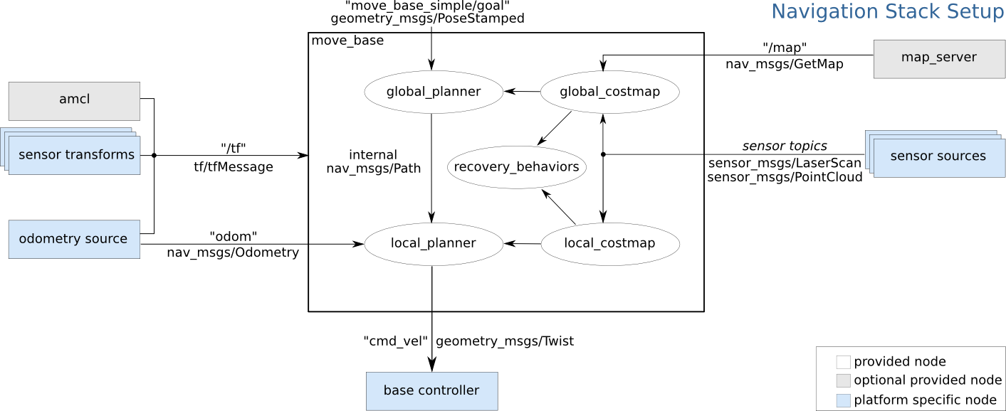
The move_base node is quite a complicated component because it implements as many as 5 closely related functionalities:

Creates a global cost map.
Determines the optimal trajectories based on the global cost map.
Creates a local cost map.
Performs temporary control based on the local cost map.
Recovery mode - determines how the robot should behave when the robot gets stuck.

Below is a diagram that contains all the elements discussed inside. On the right and left are the components that must (blue rectangles) or should be provided (grey rectangles) for the path planning algorithm to work. At the top we have information about the name of the message that starts the path planning procedure. This message triggers the so-called action - asynchronous call to another node's function (asynchronous means you don't have to wait for the procedure to finish, so you can do other things at any time). The output is a geometry_msgs/Twist message returning a velocity vector.

For all these functionalities to work properly, dozens of parameters must be properly configured. If you don't, your robot may move very counter-intuitively and even refuse to follow a certain trajectory. Configuring all these parameters is not easy, but who does not fight, does not drink champagne... or in our case, does not drive a ROSbot! 🏎️

Configure `move_base`

It is a known and good practice to store all parameters in a separate configuration folder. It used to be called config. Inside this folder I will place 6 configuration files with the extension .yaml. They will be:

costmap_common.yaml - contains parameters for local and global maps
costmap_global.yaml - contains parameters only for the global cost map
costmap_local.yaml - contains parameters only for the local cost map
planner_global.yaml - contains parameters for planning the local trajectory
planner_local.yaml - contains parameters for planning the global trajectory
move_base.yaml - contains parameters for the general behavior of the package including recovery behaviour.

Configuration note

Note that the configuration files shown below are dedicated to ROSbot 2R and may be slightly changed depending on the user's preferences or the environment in which the robot moves. For other robots, there may be a need to fine-tune these parameters individually.

Cost map

A cost map is a grid map where each cell is assigned a specific value - cost. The cost is related to the distance from the obstacle, the closer the object is, the higher the cost of a given cell on the map. We will create two cost maps, global and local. The global map is needed by the global planner and will be used to determine the shortest path from point A to point B based on historical data provided from the map and sensors. The local map, in turn, is needed by the local planner to find the best control over a section of the path.

note

If you ask yourself: "Okay, but why two maps? Wouldn't the algorithm work on one map?". I'm in a hurry to answer now. That's right, the algorithm could work. However, by splitting it into two maps, the local map can react differently to objects that appear. In addition, breaking the algorithm into two maps can improve the speed of the algorithm by reducing the local map and reducing the frequency of updating the global map.

Let's configure cost maps. To do this, create 3 configuration files in the tutorial pkg/config directory. These will be: costmap_common.yaml, costmap_global.yaml and costmap_local.yaml.

Cost map - common parameters

The first should contain common parameters for both maps, such as:

~/ros_ws/src/tutorial_pkg/config/costmap_common.yaml
# Reff: http://wiki.ros.org/costmap_2d
global_frame: map
robot_base_frame: base_link
footprint: [[0.14, 0.14], [0.14, -0.14], [-0.14, -0.14], [-0.14, 0.14]]
rolling_window: true

inflation_radius: 0.5
cost_scaling_factor: 4.0

track_unknown_space: true
observation_sources: scan
scan: {sensor_frame: laser, data_type: LaserScan, topic: scan, marking: true, clearing: true}

The code explained

global_frame - defines name of frame which contains occupancy grid map (created in previous tutorial).
robot_base_frame - defines name of robot base.
footprint - defines the outline of the robot base (robot size).
rolling_window - parameter setting parameter to true select robot_base_frame as a middle of the cost map.
inflation_radius - determines from what distance from the obstacle, take into account the cost - any distance less than indicated will be included as an additional cost.
cost_scaling_factor - defines the rate of cost decay with distance. Increasing the value causes the cost at the same distance from the obstacle to have a higher cost value
track_unknown_space - true value add a third value on the cost map unknown, if the data from the sensor does not cover part of the area e.g. an unknown value will appear around the corner, as long as we do not cross the corner of the wall.
observation_sources - define properties of used sensor, these are:

sensor_frame - name of sensor frame

data_type - type of message published by sensor (supported: PointCloud, PointCloud2, LaserScan)

topic - name of topic where sensor data is published

marking - true if sensor can be used to mark area as occupied

clearing - true if sensor can be used to mark area as clear

Cost map - global & local parameters

Next, we configure specific parameters for the local map and separate ones for global maps. The costmap_global.yaml should contains:

~/ros_ws/src/tutorial_pkg/config/costmap_global.yaml
# Reff: http://wiki.ros.org/costmap_2d
global_costmap:
    update_frequency: 2.0
    publish_frequency: 1.0

    obstacle_range: 5.0
    raytrace_range: 5.0
    static_map: true

    width: 15.0
    height: 15.0

And costmap_local.yaml should contains:

~/ros_ws/src/tutorial_pkg/config/costmap_local.yaml
# Reff: http://wiki.ros.org/costmap_2d
local_costmap:
    update_frequency: 5.0
    publish_frequency: 2.0

    obstacle_range: 2.5
    raytrace_range: 2.5
    static_map: false

    width: 2.5
    height: 2.5
    resolution: 0.02

The code explained

local_costmap/global_costmap - specifies a namespace to specify local and global map parameters. By using namespaces, it is possible to combine two files into one.
update_frequency - defines frequency in Hz for the map to be updated.
publish_frequency - defines frequency in Hz for the map to be publish display information.
obstacle_range - determines the maximum range sensor reading that will result in an obstacle being put into the costmap.
raytrace_range - defines the maximum range in which the map data will be included in the cost map.
static_map - reads the data transferred from the occupancy map.
width & height - parameters define size of map (in meters).
resolution - resolution of the cost map.

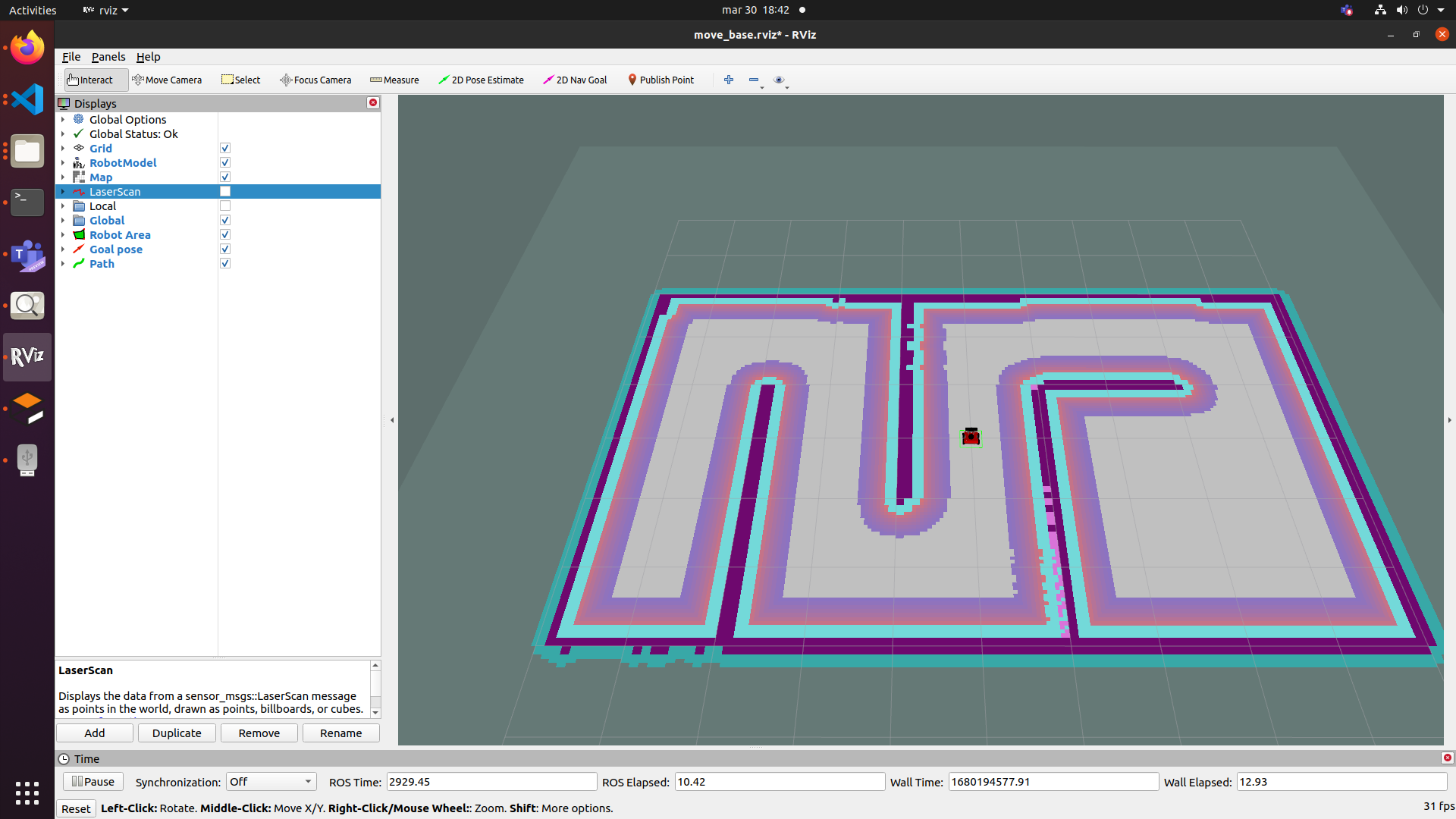
How to interpret visualization

When we run our final project, we will see a cost map. An example look can be seen in the picture below. As you can see, there are several colors on it and each of them has a specific meaning.

pink means a certain collision
cyan indicates probable collision
colors from red to blue indicate the value of the cost. High value red, low value blue.

The cost map should look like this.

Planner

The task of the planner is to attempt to reach the target position within the tolerance specified by the user. The planner is based on the cost map and creates a trajectory that goes through the cells with the lowest cost. In node move_base two planners are used: local and global. According to the global one, it is to find the optimal path based on the created global cost matrix. The local planner selects control in such a way as to get as close to the local minimum as possible.

Global planner

navfn/NavfnROS will be used as the global planner. This global planner is based on the Dikstra algorithm and is relatively simple, so there is no need to change the parameters. In the planner_global.yaml file, we will only specify the choice of the appropriate solver. For the rest of the solvers, see the nav_core documentation.

~/ros_ws/src/tutorial_pkg/config/planner_global.yaml
# Reff: http://wiki.ros.org/navfn
base_global_planner : navfn/NavfnROS

Local planner

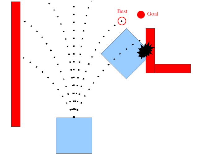
base_local_planner/TrajectoryPlannerROS will be used as the local planner. This local scheduler is based on the Dynamic Window Approach (DWA) algorithm. This is a relatively simple algorithm that first creates random velocity vectors and then simulates which velocity vector will give the best result. This result will be transferred to the wheels. The figure below illustrates the principle of operation of the algorithm:

Configuring this local scheduler is a much more difficult task due to the number of parameters available. planner_local.yaml should contain:

~/ros_ws/src/tutorial_pkg/config/planner_local.yaml
# Reff: http://wiki.ros.org/base_local_planner
base_local_planner: base_local_planner/TrajectoryPlannerROS

TrajectoryPlannerROS:
    min_vel_x: 0.1
    max_vel_x: 0.3
    min_vel_theta: -0.7
    max_vel_theta: 0.7
    min_in_place_vel_theta: 0.4
    escape_vel: -0.1

    acc_lim_theta: 1.0
    acc_lim_x: 1.0

    holonomic_robot: false

    xy_goal_tolerance: 0.1
    yaw_goal_tolerance: 0.2

    meter_scoring: true
    path_distance_bias: 20
    goal_distance_bias: 15
    occdist_scale:  0.01

    sim_time: 2.0

The code explained

TrajectoryPlannerROS - namespace depends on the type of planner.
min_vel_x - defines minimum linear velocity that will be set by trajectory planner. This should be adjusted to overcome rolling resistance and other forces that may suppress robot from moving.
max_vel_x - defines maximum linear velocity that will be set by trajectory planner.
max_vel_theta & min_vel_theta - defines maximum and minimum angular velocity that will be set by trajectory planner.
min_in_place_vel_theta - defines minimum angular velocity that will be set by trajectory planner. This should be adjusted to overcome rolling resistance and other forces that may suppress robot from moving.
acc_lim_theta & acc_lim_x - parameters define maximum values of accelerations used by trajectory planner.
holonomic_robot - defines if robot is holonomic.
meter_scoring - defines if cost function arguments are expressed in map cells or meters (if true, meters are considered).
xy_goal_tolerance & yaw_goal_tolerance - parameters define how far from destination it can be considered as reached. Linear tolerance is in meters, angular tolerance is in radians.
path_distance_bias, goal_distance_bias & occdist_scale - a group of parameters defines how much the aspect related to keeping to the path, following to the local minimum and avoiding objects should affect the selection of the trajectory.
sim_time - the amount of time to forward-simulate trajectories in seconds

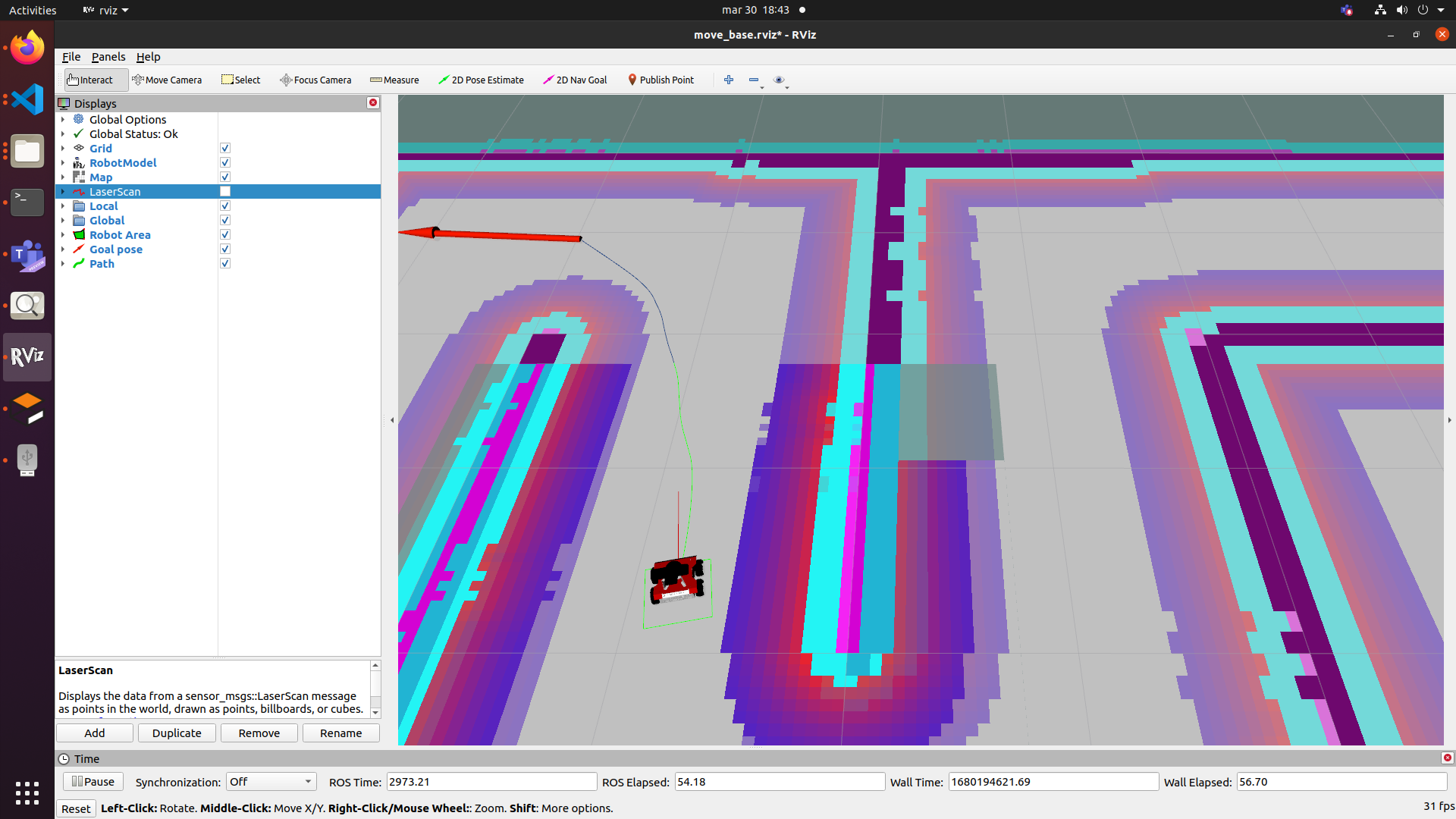
How to interpret visualization?

Once we run our project, we will see 3 paths in RViz. You can see them in the picture below. The global path is marked in blue. The local path is also marked in green, but only the part of it that is on the local map. In red is the local path that the robot is following at the moment.

Configuration `move_base`

The last thing is to configure the move_base node itself. It contains basic information about the node as well as parameters related to recovery mode. So we create the last file move_base.yaml and enter the following parameters into it.

~/ros_ws/src/tutorial_pkg/config/move_base.yaml
# Reff: http://wiki.ros.org/move_base
recovery_behavior_enabled: true

controller_frequency: 10.0
controller_patience: 10.0
planner_frequency: 5.0
planner_patience: 5.0

conservative_reset_dist: 6.0
oscillation_timeout: 10.0
oscillation_distance: 0.15

The code explained

recovery_behavior_enabled - enable or disable the move_base recovery behaviors to attempt to clear out space.
controller_frequency - defines the rate in Hz at which to run the control loop and send velocity commands to the base.
controller_patience - defines how long the controller will wait in seconds without receiving a valid control before space-clearing operations are performed.
planner_frequency - defines the rate in Hz at which to run the global planning loop.
planner_patience - how long the planner will wait in seconds in an attempt to find a valid plan before space-clearing operations are performed.
conservative_reset_dist - defines the distance away from the robot in meters beyond which obstacles will be cleared from the costmap when attempting to clear space in the map.
oscillation_timeout - defines how long in seconds to allow for oscillation before executing recovery behaviors.
oscillation_distance - defines how far in meters the robot must move to be considered not to be oscillating. Moving this far resets the timer.

Launching path planning node

Ugh, I know that it was not easy to go through all these parameters, but thanks to this we are getting closer to the most pleasant one, i.e. starting autonomous driving in the robot. To test above configuration you will need to run move_base node along with localization.launch, which we created in previous tutorial.

To sum up, you will need to run following nodes:

ROSbot/Gazebo - turn on the robot, calculate odometry, and publish and subscribe all necessary to move the robot,
rplidarNode - driver for rpLidar laser scanner,
amcl - localization node,
map_server - to load the map,
move_base - trajectory planner,
rviz - visualization tool.

For the move_base node you will need to specify paths to already created .yaml configuration files. This is shown in the following launch file:

~/ros_ws/src/tutorial_pkg/launch/move_base.launch
<launch>

   <arg name="use_gazebo" default="false" />
   <arg name="map_name" default="map.yaml"/>

   <!-- Localization -->
   <include file="$(find tutorial_pkg)/launch/localization.launch">
      <arg name="use_gazebo" value="$(arg use_gazebo)" />
      <arg name="map_name" default="$(arg map_name)"/>
   </include>

   <!-- Path planning -->
   <node pkg="move_base" type="move_base" respawn="false" name="move_base" output="screen">
      <rosparam file="$(find tutorial_pkg)/config/move_base.yaml" command="load" />
      <rosparam file="$(find tutorial_pkg)/config/costmap_common.yaml" command="load" ns="global_costmap" />
      <rosparam file="$(find tutorial_pkg)/config/costmap_common.yaml" command="load" ns="local_costmap" />
      <rosparam file="$(find tutorial_pkg)/config/costmap_global.yaml" command="load" />
      <rosparam file="$(find tutorial_pkg)/config/costmap_local.yaml" command="load" />
      <rosparam file="$(find tutorial_pkg)/config/planner_global.yaml" command="load" />
      <rosparam file="$(find tutorial_pkg)/config/planner_local.yaml" command="load" />
   </node>

   <node pkg="rviz" type="rviz" name="rviz" args="-d $(find tutorial_pkg)/rviz/move_base.rviz"/>

</launch>

The code explained

<rosparam file="$(find tutorial_pkg)/config/move_base.yaml" command="load" />

Load move_base parameters.

<rosparam file="$(find tutorial_pkg)/config/costmap_common.yaml" command="load" ns="global_costmap" />
<rosparam file="$(find tutorial_pkg)/config/costmap_common.yaml" command="load" ns="local_costmap" />

Load common parameters to global and local cost maps with appropriate namespace.

<rosparam file="$(find tutorial_pkg)/config/costmap_global.yaml" command="load" />
<rosparam file="$(find tutorial_pkg)/config/costmap_local.yaml" command="load" />
<rosparam file="$(find tutorial_pkg)/config/planner_global.yaml" command="load" />
<rosparam file="$(find tutorial_pkg)/config/planner_local.yaml" command="load" />

Load the remaining parameters for: global & local cost map and for: global & local planner.

Setting goal for trajectory planner

Before we run move_base.launch, we have configured RViz for you. Download this RViz configuration move_base.rviz. Name the file as move_base.rviz and place it in the tutorial_pkg/rviz directory. Now we are ready to launch our autonomous driving program.

ROSbot
Gazebo simulator

husarion@husarion:~$

docker compose up -d rosbot ros-master rplidar
roslaunch tutorial_pkg move_base.launch

user@mylaptop:~$

roslaunch tutorial_pkg move_base.launch use_gazebo:=true

After you launched trajectory planner with all accompanying nodes, your robot still will not be moving anywhere. You have to specify target position first. To set goal position for robot click on 2D nav goal button from Toolbar, then click a place in Visualization window, that will be destination for your robot. Observe as path is generated (you should see a line from your robot pointing to direction) and robot is moving to its destination. It should look like this:

Task 1

Add an obstacle and watch how the robot copes.

Task 2

We encourage you to change the parameters and check the result. If you are not sure what parameter are worth to change try some of these: inflation_radius, sim_time, static_map, min_in_place_vel_theta.

Summary

Congratulations, all the knowledge gained so far has allowed you to create your own autonomous robot! After completing this tutorial, you should be able to configure the move_base node to plan trajectories for your robot. You should also understand how to interpret the results in RViz. Most importantly, you can set a target target for your robot and it will do the rest! I hope you managed to configure everything correctly despite the hardships. In the next and final tutorial we will use ROSbot to patrol our area.

by Łukasz Mitka, Rafał Górecki, Husarion

Do you need any support with completing this tutorial or have any difficulties with software or hardware? Feel free to describe your thoughts on our community forum: https://community.husarion.com or to contact with our support: support@husarion.com

Chapter description​

Introduction​

Graph methods​

Occupancy grid methods​

Path planning in ROS​

Introduction to move_base​

Configure move_base​

Cost map​

Cost map - common parameters​

Cost map - global & local parameters​

Planner​

Global planner​

Local planner​

Configuration move_base​

Launching path planning node​

Setting goal for trajectory planner​

Summary​

Chapter description

Introduction

Graph methods

Occupancy grid methods

Path planning in ROS

Introduction to `move_base`

Configure `move_base`

Cost map

Cost map - common parameters

Cost map - global & local parameters

Planner

Global planner

Local planner

Configuration `move_base`

Launching path planning node

Setting goal for trajectory planner

Summary