Navigation
In this tutorial, you will learn the basics of navigation. For this purpose, the popular and powerful nav2 package will be used. Thanks to the knowledge gained in this and previous chapters, functionality will be implemented that enables the creation of an autonomous robot capable of reaching any location on the map. The chapter is quite challenging, so we encourage you to work through this material when you are well-rested.
Prerequisites
This tutorial is dedicated to the ROSbot XL equipped with any Slamtec LiDAR and you will also need to have a computer with ROS installed, which will be used for data visualization. However, most of the information and commands are also compatible with ROSbot 2R, and most changes are simple and come down to launching the appropriate container, depending on your hardware configuration. It is also possible to follow the tutorial using the Gazebo simulation.
Due to the older distribution of the ROS Foxy operating system on ROSbot 2 PRO, the following tutorial will not work, but you can achieve the same effect as on other robots using the rosbot-autonomy demo.
If you don't already own a ROSbot, you can get one from the Husarion store.
The tutorials are designed to flow sequentially and are best followed in order. If you're looking to quickly assess the content of a specific tutorial, refer to the ROS 2 Tutorials repository, which contains the completed outcomes.
Requirements
This tutorial will be based on the knowledge from the previous chapters, so make sure that the following topics are familiar to you:
- Tutorial 4: How to control the robot?
- Tutorial 7: How information about the mutual position of objects is published?
- Tutorial 8: What is and how to receive data from a LiDAR/laser scanner?
- Tutorial 8: How to create and upload a map?
- Tutorial 8: How to locate the robot on the map?
Introduction
Robot navigation consists in determining the sequence of maneuvers that the robot must perform in order to move from the starting point to the destination, while avoiding collisions with obstacles. Navigation can be simplified to three main algorithms: costmap, planner and controller.
It can be compared to driving a car with the navigation turned on. Navigation will show us the optimal way to the destination, but we, as drivers, can react to situations on the road. For example, if you see a traffic jam, you can try to avoid it even though the navigation tells us to go straight.
Costmap
Costmap is similar to the map a robot uses to find out where it can safely go. Imagine that you are trying to get through a room full of obstacles such as furniture and toys. The costmap helps the robot understand which areas are easy to navigate and which are a bit more difficult.
The costmap is created based on the provided map and data from sensors such as cameras and laser scanners that measure whether there are obstacles in the way. Then it creates a special map where each spot has a "cost" value. Low cost means it is safe to move there, high cost means congested or blocked area.
Planner
Planner, also known as the global planner or just path planer, is therefore responsible for determining the optimal path to the goal. The planner uses a costmap to get you to your destination safely and quickly. It avoids high-cost areas, such as obstacles, and prefers low-cost areas, such as open spaces. This helps the robot make smart decisions about where to move. Some of the most popular scheduling algorithms are: Dijkstra’s algorithm, A*, D*, Artificial potential field method, Visibility graph method. All of these path planning algorithms are based on one of two approaches.
- Graph methods - method that is using graphs, defines places where robot can be and possibilities to traverse between these places. In this representation graph vertices define places e.g. rooms in building while edges define paths between them e.g. doors connecting rooms. Moreover each edge can have assigned weights representing difficulty of traversing path e.g. door width or energy required to open it. Finding the trajectory is based on finding the shortest path between two vertices while one of them is robot current position and second is destination.
- Occupancy grid methods - method that is using occupancy grid divides area into cells (e.g. map pixels) and assign them as occupied or free. One of cells is marked as robot position and another as a destination. Finding the trajectory is based on finding shortest line that do not cross any of occupied cells.
Controller
Controller, also known as the local planner, is responsible for taking actions that will allow you to get closer to the goal, while taking into account the current state of the path. There are many types of controllers. The one we're going to use is called Regulated Pure Pursuit.
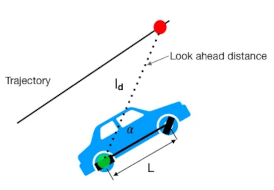
Regulated Pure Pursuit is a path tracking algorithm. Its basic principle is to continuously select a destination on a predetermined path and adjust the vehicle's steering angle to guide it towards that point. This is achieved by defining the path as a sequence of waypoints and specifying a lookahead distance. The algorithm tries to minimize the lateral distance between the current position of the vehicle and the point on the route. Using trigonometry, it calculates the necessary steering angle to steer the vehicle towards that target, and the vehicle's control system adjusts accordingly.
Navigation in ROS
In ROS it is possible to plan a path based on the occupancy map created in previous chapter, created with the slam_toolbox node. The next step is to add a navigation package that will allow you to safely move around the entire map. In the first step, you will specify the parameters used to create the costmap, on the basis of which the optimal trajectory will be selected. Knowing the best trajectory, you can choose the control that will allow you to travel the designated path as quickly as possible. In ROS, both of these functions: determining the optimal path and determining the appropriate speed values can be done using the nav2 package.
Introduction to nav2
The nav2 node is quite a complicated component because it implements as many closely related functionalities:
- Planner Server - creates a global costmap and determines the optimal trajectories based on the global costmap.
- Controller Server - creates a local costmap and implements the server for handling the controller requests.
- Behavior Server - determines the actions that should be performed when the robot gets stuck.
- BT Navigator Server - behavioral tree determining the execution of the appropriate step of the algorithm (e.g. first determine the optimal path and then run the controller).
- Smoother Server - creates smoother path plans to be more continuous and feasible.
Below is a diagram that contains all discussed elements inside blue area.
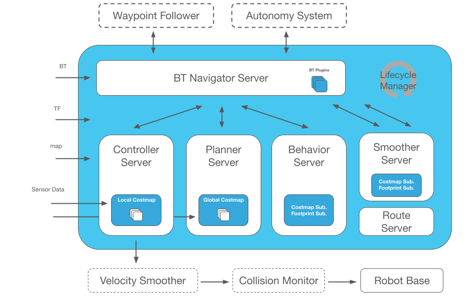
On the left are the components that must be provided for the nav2 algorithm to work. These are:
- BT allows you to change the behavior of services to create a unique robot behavior (default behavior tree will be used),
- TF is necessary to determine the relative position between frames. For example, between LiDAR, the base of the robot, and the map, so you can uniquely determine the location of the obstacle detected by LiDAR relative to the map,
- map is essential at the stage of planning the path and determining the optimal path,
- Sensor Data sensor data is necessary to react to changes occurring in the robot's local vicinity. The controller is able to dynamically avoid new objects that are not on the map.
In addition, nav2 encourages, but does not require configuration of additional functionalities, such as: Waypoins Follower, Autonomy System, Velocity Smoother, Collision Monitor. For all these functionalities to work properly, dozens of parameters must be properly configured. If you don't, your robot may move very counter-intuitively and even refuse to follow a certain trajectory, so we'll focus primarily on Planner Server and Controller Server.
Configuring these two Servers alone is not easy, but who does not fight, does not drink champagne ... or in our case, does not drive a ROSbot! 🏎️
Configure nav2
The configuration of nav2 is a very difficult task, because it is based on many advanced algorithms, where each particular algorithm contains a number of its own parameters and functions. Discussing all these parameters would be very time consuming, so in order to start navigation, download or copy the configuration from github. Place the configuration file named navigation.yaml inside the path tutorial_pkg/config. Inside this file is the configuration of several services:
amcl- parameters for localization algorithm learned in previous chapter used to locate the robot on the map,behavior_server- parameters to configure recovery behavior,bt_navigator- parameters for the behavioral tree,controller_server- parameters related to the selection and fine-tuning of the controller,local_costmap/global_costmap- parameters responsible for creating a local/global costmap,planner_server- parameters related to the selection and fine-tuning of the global path,waypoint_follower- parameters related to following a multi-point route,velocity_smoother- parameters to smooth out the robot's motion.
File created based on official Nav2 Documentation where you can found more information.
Please note that the configuration file presented below is dedicated to ROSbot XL. If a different robot is used, some parameters may need to be adjusted individually.
Parameters overview
Costmap
A costmap is a grid map where each cell is assigned a specific value - cost. The cost is related to the distance from the obstacle, the closer the object is, the higher the cost of a given cell on the map. You will create two costmaps, global and local. The global map is needed by the global planner and will be used to determine the shortest path from point A to point B based on historical data provided from the map and sensors. The local map, in turn, is needed by the local planner to find the best control over a section of the path.
If you ask yourself: "Okay, but why two maps? Wouldn't the algorithm work on one map?". I'm in a hurry to answer.
That's right, the algorithm could work. However, by using two maps, the number of operations of the algorithm can be limited. The global map is used primarily to determine the global path, while the local map is used to react to nearby objects and follow the global path.
To remember
Among the dozens of parameters related to the map, it is worth remembering the existence of:
update_frequency- defines frequency in Hz for the map to be updated,publish_frequency- defines frequency in Hz for the map to be publish display information,global_frame- defines name of frame which contains occupancy grid map (created in previous tutorial),robot_base_frame- defines name of robot base,footprint/robot_radius- defines the outline of the robot base (robot size),footprint_padding- defines amount to pad footprint (m).rolling_window- parameter setting parameter to true selectrobot_base_frameas a middle of the costmap,inflation_radius- determines from what distance from the obstacle, take into account the cost - any distance less than indicated will be included as an additional cost,cost_scaling_factor- defines the rate of cost decay with distance, increasing the value causes the cost at the same distance from the obstacle to have a higher cost value,obstacle_max_range- determines the maximum range sensor reading that will result in an obstacle being put into the costmap,width&height- parameters define size of map (for local map),track_unknown_space-truevalue add a third value on the costmap unknown, if the data from the sensor does not cover part of the area e.g. an unknown value will appear around the corner, as long as we do not cross the corner of the wall (for global map),resolution- resolution of the costmap,observation_sources- define properties of used sensor, these are:data_type- type of message published by sensor (supported:PointCloud,PointCloud2,LaserScan),topic- name of topic where sensor data is published,marking-trueif sensor can be used to mark area as occupied,clearing-trueif sensor can be used to mark area as clear.
How to interpret visualization
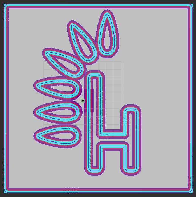
When you run our navigation project, you will see a costmap. An example look can be seen in the picture below. As you can see, there are several colors on it and each of them has a specific meaning:
- pink inside cyan means a wall = certain collision,
- cyan indicates high probable collision,
- colors from red to blue indicate the value of the cost. Red means high value (the wall is close), blue means low value (the wall is far away).
The costmap should look like this:
Planner
The planner's task is to find a way to get to the destination. The planner relies on the costmap and finds a trajectory to get there. Navfn Planner will be used as the global planner. This global planner, depend on configuration is based on the Dikstra or A* algorithm depend on use_astar parameter. Configuration of Navfn Planner is relatively simple, there is probably no need to change parameters. Click on the following links if you want to know more about the Planner Server or Navfn Planner configuration.
To remember
Besides NavFn Planner, there are other planners like Smac Planner and Theta Star Planner. Feel free to use them. Using Navfn Planner it is worth remembering the existence of use_astar parameter.
Controller
The configuration of Navfn Planner is simple due to the small number of parameters. Unfortunately, the configuration of the controller may take longer due to the large number of parameters. Regulated Pure Pursuit will be used for control. Click on the following links if you want to know more about the Controller Server or Regulated Pure Pursuit configuration. You can learn how the Pure Pursuit algorithm works in this video.
To remember
Besides Regulated Pure Pursuit, there are other planners like DWB Controller and Model Predictive Path Integral Controller. The DWB Controller is relatively easy to understand so it may take more time to properly configure and understand the Model Predictive Path Integral Controller.
Using Regulated Pure Pursuit it is worth remembering the existence of:
desired_linear_vel- the desired maximum linear velocity (m/s) to use,min_lookahead_dist/max_lookahead_dist- the minimum/maximum lookahead distance (m) threshold,rotate_to_heading_min_angle- the difference in the path orientation and the starting robot orientation (radians) to trigger a rotate in place (only ifuse_rotate_to_headingparam istrue),rotate_to_heading_angular_vel- the speed of rotation, ifuse_rotate_to_headingparam istrue.
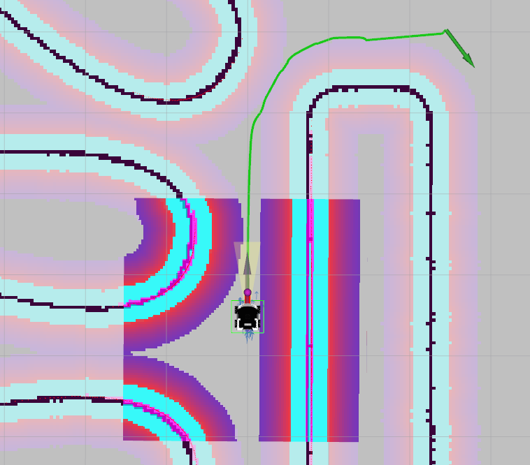
How to interpret visualization
After running our project, RViz will launch, as in the picture below, where you can observe a green path and a red line at the end of which there is a purple point. As you can easily guess, the green path is a global trajectory. The purple point is the point to which you can determine the controls that will allow you to approach the indicated point. The red line defines the collision distance, which, if exceeded, will slow down or stop the vehicle.
Launching navigation
We've finally gone through all these parameters. The last step is to create a launch file that will launch the nav2 nodes that will allow you to do autonomous driving. In the launch folder, create a new file named localization.launch.py. This file will contain:
- definition of three parameters:
map,use_sim_time,params_file, - run
nav2_bringup, - launching RViz in a specific configuration.
from launch import LaunchDescription
from launch.actions import DeclareLaunchArgument, IncludeLaunchDescription
from launch.launch_description_sources import PythonLaunchDescriptionSource
from launch.substitutions import LaunchConfiguration, PathJoinSubstitution
from launch_ros.substitutions import FindPackageShare


def generate_launch_description():
    tutorial_dir = FindPackageShare('tutorial_pkg')
    nav2_bringup_launch_file_dir = PathJoinSubstitution(
        [FindPackageShare('nav2_bringup'), 'launch', 'bringup_launch.py']
    )

    map_yaml_file = LaunchConfiguration('map')
    params_file = LaunchConfiguration('params_file')
    use_sim_time = LaunchConfiguration('use_sim_time')

    declare_map_yaml_cmd = DeclareLaunchArgument(
        'map',
        default_value=PathJoinSubstitution([tutorial_dir, 'maps', 'map.yaml']),
        description='Full path to map yaml file to load',
    )

    declare_params_file_cmd = DeclareLaunchArgument(
        'params_file',
        default_value=PathJoinSubstitution([tutorial_dir, 'config', 'navigation.yaml']),
        description='Full path to the ROS2 parameters file to use for all launched nodes',
    )

    declare_use_sim_time_cmd = DeclareLaunchArgument(
        'use_sim_time', default_value='false', description='Use simulation (Gazebo) clock if true'
    )

    nav2_bringup_launch = IncludeLaunchDescription(
        PythonLaunchDescriptionSource([nav2_bringup_launch_file_dir]),
        launch_arguments={
            'map': map_yaml_file,
            'params_file': params_file,
            'use_sim_time': use_sim_time,
        }.items(),
    )

    return LaunchDescription(
        [
            declare_map_yaml_cmd,
            declare_params_file_cmd,
            declare_use_sim_time_cmd,
            nav2_bringup_launch,
        ]
    )
Run RViz on your private computer for visualization. If you don't know how to do it, check the RViz Visualization
- ROSbot
- Gazebo simulator
Run the ROSbot.
docker compose up -d microros <rosbot_service> rplidar
How to add RPlidar to your configuration?
You can add rplidar service to your compose.yaml by placing following code at the end of file.
rplidar:
    image: husarion/rplidar:humble
    <<: *net-config
    devices:
    - /dev/ttyRPLIDAR:/dev/ttyUSB0
    command: ros2 launch sllidar_ros2 sllidar_launch.py serial_baudrate:=${LIDAR_BAUDRATE:-115200}
Depend on your ROSbot model, you should use appropriate name for your
<rosbot_service>. To check available docker service use following commanddocker compose config --services, or find suitable Docker images prepared by Husarion.
Then in the new terminal run navigation.launch.py.
ros2 launch tutorial_pkg navigation.launch.py
In the case of Rosbot 2R and PRO, it is necessary to change the name of the topic /scan_filtered to /scan in all configuration files. Due to the size of the ROSbot XL, it is necessary to remove all laser reflections that hit the robot's elements, such as the camera handle.
Running the simulator is very easy thanks to the created aliases. If you haven't done so already check configure your environment.
ROSBOT_SIM
Then in the new terminal run navigation.launch.py.
ros2 launch tutorial_pkg navigation.launch.py use_sim_time:=True
Run RViz for visualization according to this instruction.
Setting destination goal
After booting with nav2 you should see RViz. Your robot should be on the map. To start navigation, you must first specify a destination. To set a target position for your robot, click the "Nav2 Goal" button in the toolbar, then click on the location in the "Visualization Window" that will be the destination for your robot. Watch the robot move along the generated path (you should see a line from the robot pointing in the direction). Sample result:
- ROSbot
- Gazebo simulator
Task 1
Add an obstacle and watch how the robot copes.
Task 2
Test Waypoint mode. For example, try to loop around the entire map and return to the starting point.
Task 3
We encourage you to change the parameters and check the result. For example try to make the robot drive closer to the walls and decrease velocity speed for safety.
Details
Hint
Parameter names that may be useful:desired_linear_vel, footprint_padding, inflation_radius, cost_scaling_factorSummary
Congratulations, all the knowledge gained so far has allowed you to create your own autonomous robot! After completing this tutorial, you should be able to configure the nav2 node to plan trajectories for your robot. You should also understand how to interpret the results in RViz. Most importantly, you can set a target for your robot and it will do the rest! I hope you managed to configure everything correctly despite the hardships. In the next and final tutorial we will use ROSbot to patrol our area.
Since the creation of these tutorials, improvements have been made to enhance navigation quality. You can find the latest demos for our robots at the following links:
by Rafał Górecki, Husarion
Need help with this article or experiencing issues with software or hardware? 🤔
- Feel free to share your thoughts and questions on our Community Forum. 💬
- To contact service support, please use our dedicated Issue Form. 📝
- Alternatively, you can also contact our support team directly at: support@husarion.com. 📧