SLAM
In this tutorial, we will walk you through the map creation process and discuss the SLAM algorithm, which consists of two parts: mapping and localization. For this purpose, I will use the package slam_toolbox, which will be used to create a terrain map. Terrain mapping is usually a necessary element to create more advanced autonomous driving systems. In addition, thanks to the knowledge of the map and knowing that it does not change, we can use simple location algorithms such as amcl, which compares the current data from the sensors and tries to adjust the location in such a way that the readings from the point cloud match the map. To do this, we will use the LIDAR mounted on board our ROSbot.
Prerequisites
This tutorial is dedicated to the ROSbot XL equipped with any Slamtec LiDAR and you will also need to have a computer with ROS installed, which will be used for data visualization. However, most of the information and commands are also compatible with ROSbot 2R/2 PRO, and most changes are simple and come down to launching the appropriate container, depending on your hardware configuration. It is also possible to solve the tutorial using the Gazebo simulation.
If you don't already own a ROSbot, you can get one from the Husarion store.
The tutorials are designed to flow sequentially and are best followed in order. If you're looking to quickly assess the content of a specific tutorial, refer to the ROS 2 Tutorials repository, which contains the completed outcomes.
Introduction
SLAM (simultaneous localization and mapping) is a technique for creating a map of environment and determining robot position at the same time. It is widely used in robotics. While moving, current measurements and localization are changing, in order to create map it is necessary to merge measurements from previous positions.
To perform an accurate and precise SLAM, one of the simplest solutions is to use a laser scanner and an odometry system (speed measurement system based on encoder data). However, due to the imperfections of the sensors, the map creation process is much more difficult. Why? Because various imperfections, e.g. caused by wheel slippage, can cause the same wall to be classified as two objects. To counteract unwanted changes, these algorithms use various tricks, such as the Monte Carlo method, which will be described in detail in Localize robot part, where you will use amcl algorithm. Note, however, that the slam_toolbox algorithm also performs similar operations to improve the quality of the map. For more details with explanations about how SLAM works check this video.
Laser scanner
In this example we will use RPLIDAR (laser scanner). For ROSbot, you can find a repository online containing rplidarNode from the rplidar_ros package to run RPLIDAR, but using a prepared docker is much simpler. The container will automatically configure and run rplidarNode. Upon startup, the node sends scans to topic /scan with a message of type sensor_msgs/LaserScan.
To test your sensor works type:
- ROSbot
- Gazebo simulator
Running the ROSbot is very easy thanks to the created docker services.
docker compose up -d microros <rosbot_service> rplidar
How to add RPlidar to your configuration?
You can add rplidar service to your compose.yaml by placing following code at the end of file.
rplidar:
    image: husarion/rplidar:humble
    <<: *net-config
    devices:
    - /dev/ttyRPLIDAR:/dev/ttyUSB0
    command: ros2 launch sllidar_ros2 sllidar_launch.py serial_baudrate:=${LIDAR_BAUDRATE:-115200}
After few seconds LiDAR should start spinning and new /scan topic should appear.
Depend on your ROSbot model, you should use appropriate name for your
<rosbot_service>. To check available docker service use following commanddocker compose config --services, or find suitable Docker images prepared by Husarion.
Running the simulator is very easy thanks to the created aliases. If you haven't done so already check configure your environment.
ROSBOT_SIM
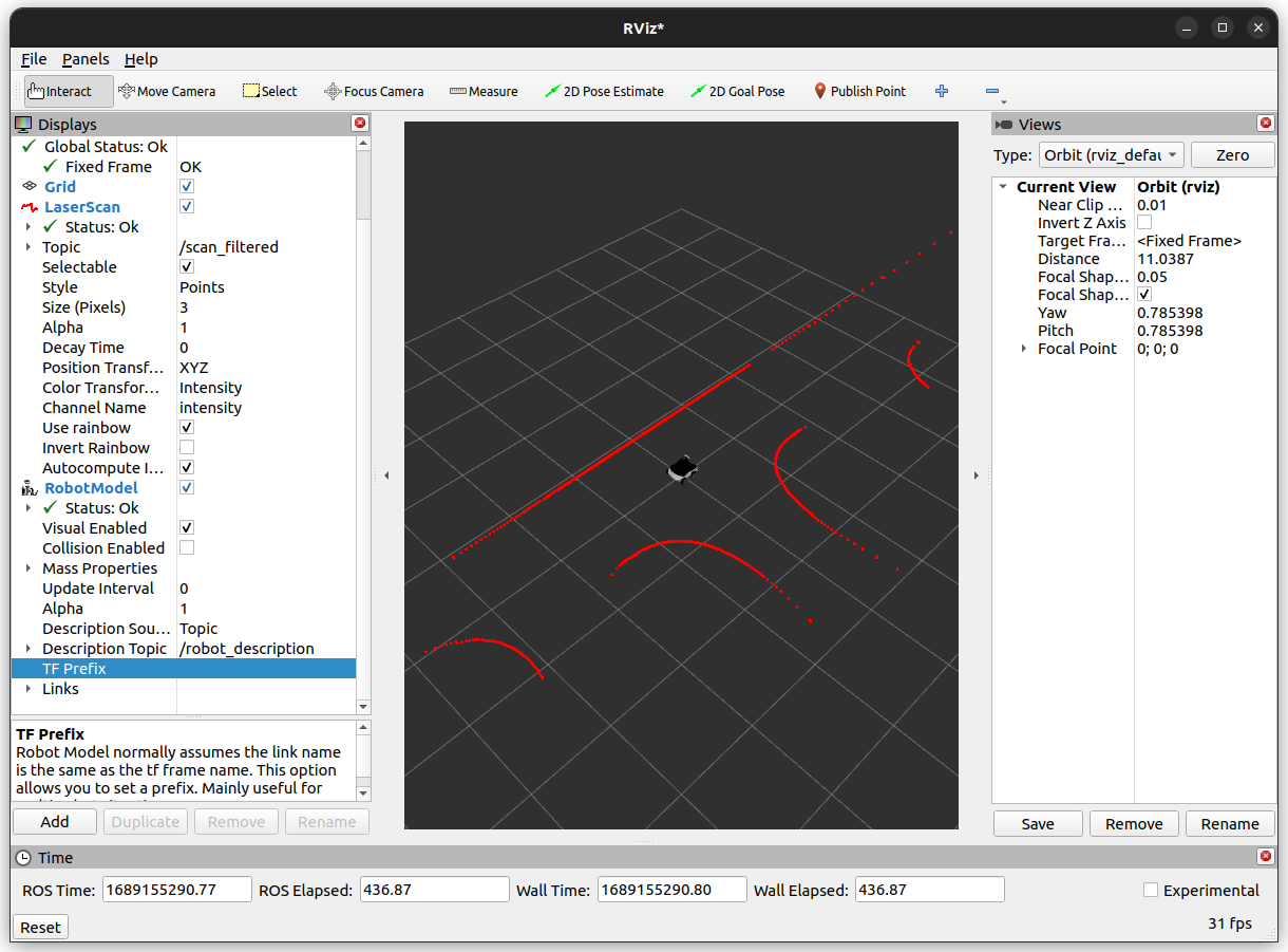
You should have /scan topic in your system. You can examine it with ros2 topic list. It is possible to echo data but you will get lots of output, which is hard to read. Better method for checking the /scan topic is to use RViz. Run RViz and click Add. In new window select By topic tab and from the list select /scan. In visualized items list find position Fixed Frame and change it to base_link. To improve visibility of scanned shape, you may need to adjust one of visualized object options, set value of Style to Points. You should see many points which resemble shape of obstacles surrounding your robot. You can also add a RobotModel in RViz listen to /robot_description topic. Enable keyboard controls and watch how environment change.
ros2 run teleop_twist_keyboard teleop_twist_keyboard
SLAM
To build the map we will use the async_slam_toolbox_node node from the slam_toolbox package. This node subscribes to the /scan_filtered topic to obtain data about the surrounding environment. In addition, it subscribes to /tf messages to obtain the position of the laser scanner and the robot relative to the starting point. Thanks to the position and laser data, the algorithm can determine the distance of the robot from the surrounding obstacles and on this basis create an occupation map. This map is published in topic /map in message nav_msgs/OccupancyGrid.
In the case of Rosbot 2R and PRO, it is necessary to change the name of the topic /scan_filtered to /scan in all configuration files. Due to the size of the ROSbot XL, it is necessary to remove all laser reflections that hit the robot's elements, such as the camera handle.
SLAM configuration
Lets start our work from downloading slam_toolbox package.
sudo apt install ros-$ROS_DISTRO-slam-toolbox
To run this node it is necessary to set parameters. There are many parameters provided by async_slam_toolbox_node node. All the parameters are in the slam_toolbox github repository, and the most important ones are described below.
base_frame- name of frame related with robot, in our case it will bebase_link,odom_frame- name of frame related with starting point, in our case it will beodom,scan_topic- name of topic with sensor data, in our case it will be/scan_filtered,resolution- resolution of the map in meters, in our case it will be set to0.04,max_laser_range- the maximum usable range of the laser, in our case it will be12.0metersmode- mapping or localization mode for performance optimizations in the Ceres problem creation
All above parameters we set in dedicated yaml file in new config folder.
slam:
  ros__parameters:

    # Plugin params
    solver_plugin: solver_plugins::CeresSolver
    ceres_linear_solver: SPARSE_NORMAL_CHOLESKY
    ceres_preconditioner: SCHUR_JACOBI
    ceres_trust_strategy: LEVENBERG_MARQUARDT
    ceres_dogleg_type: TRADITIONAL_DOGLEG
    ceres_loss_function: None

    # ROS Parameters
    odom_frame: odom
    map_frame: map
    base_frame: base_link
    scan_topic: /scan_filtered
    # mode: mapping # It will be set in launch file
    debug_logging: false
    throttle_scans: 1
    transform_publish_period: 0.02 # If 0 never publishes odometry
    map_update_interval: 2.0
    resolution: 0.04
    max_laser_range: 12.0
    minimum_time_interval: 0.1
    transform_timeout: 0.2
    tf_buffer_duration: 20.0
    stack_size_to_use: 40000000
    enable_interactive_mode: false

    # General Parameters
    use_scan_matching: true
    use_scan_barycenter: true
    minimum_travel_distance: 0.3
    minimum_travel_heading: 0.5
    scan_buffer_size: 10
    scan_buffer_maximum_scan_distance: 7.0
    link_match_minimum_response_fine: 0.1
    link_scan_maximum_distance: 1.0
    loop_search_maximum_distance: 3.0
    do_loop_closing: true
    loop_match_minimum_chain_size: 10
    loop_match_maximum_variance_coarse: 3.0
    loop_match_minimum_response_coarse: 0.35
    loop_match_minimum_response_fine: 0.45

    # Correlation Parameters - Correlation Parameters
    correlation_search_space_dimension: 0.5
    correlation_search_space_resolution: 0.01
    correlation_search_space_smear_deviation: 0.1

    # Correlation Parameters - Loop Closure Parameters
    loop_search_space_dimension: 8.0
    loop_search_space_resolution: 0.05
    loop_search_space_smear_deviation: 0.03

    # Scan Matcher Parameters
    distance_variance_penalty: 0.5
    angle_variance_penalty: 1.0
    fine_search_angle_offset: 0.00349
    coarse_search_angle_offset: 0.349
    coarse_angle_resolution: 0.0349
    minimum_angle_penalty: 0.9
    minimum_distance_penalty: 0.5
    use_response_expansion: true
You can find detailed explanation of this parameters on official Github repository
The structure of config file
The configuration file should start with the node name (in our case amcl). Note: If the name is not exactly the same as the node name, the parameters will not be loaded. After the node name, enter ros__parameters (there are two _ characters in the name). From the next line, enter the names and values of the parameters.
*If you are using namespace you should add name of namespace in the first line. Example:
namespace_name:
  node_name:
    ros__parameters:
      param1: value1
      param2: value2
      ...
Launch slam_toolbox
Then create a new file slam.launch.py which will run async_slam_toolbox_node with the configuration contained in the file.
from launch import LaunchDescription
from launch.actions import DeclareLaunchArgument
from launch.substitutions import LaunchConfiguration, PathJoinSubstitution
from launch_ros.actions import Node
from launch_ros.substitutions import FindPackageShare


def generate_launch_description():
    slam_params_file = LaunchConfiguration('slam_params_file')
    use_sim_time = LaunchConfiguration('use_sim_time')

    slam_params_file_arg = DeclareLaunchArgument(
        'slam_params_file',
        default_value=PathJoinSubstitution(
            [FindPackageShare("tutorial_pkg"), 'config', 'slam.yaml']
        ),
        description='Full path to the ROS2 parameters file to use for the slam_toolbox node',
    )

    use_sim_time_arg = DeclareLaunchArgument(
        'use_sim_time', default_value='false', description='Use simulation/Gazebo clock'
    )

    slam_node = Node(
        package='slam_toolbox',
        executable='async_slam_toolbox_node',
        name='slam',
        parameters=[slam_params_file, {'use_sim_time': use_sim_time}],
    )

    return LaunchDescription([use_sim_time_arg, slam_params_file_arg, slam_node])
Let's make one more change before we run the script. Let's create a new maps folder where we will store information about the saved map. It is still necessary to inform the compiler about the newly created folder. Add this folder to CMakeList.txt:
install(DIRECTORY
  config
  launch
  img_data
  maps
  DESTINATION share/${PROJECT_NAME})
- ROSbot
- Gazebo simulator
ros2 launch tutorial_pkg slam.launch.py
ros2 launch tutorial_pkg slam.launch.py use_sim_time:=true
RViz Visualization
To visualize data, you can use your private computer and choose one of the options below.
-
Download appropriate configuration file and run:
user@mylaptop:~$rviz2 -d <path/to/configuration.rviz> -
Build tutorial_pkg repository, amd run:
user@mylaptop:~$ros2 launch tutorial_pkg rviz.launch.py config_file:=<configuration.yaml> -
Create your own configuration.
For manually configuration run:
user@mylaptop:~$rviz2For SLAM configuration you should a add the:
/scan_filteredand/maptopics. You can select them from By topic tab.
If you want to see the robot model in rviz, it is necessary to build the rosbot package on your computer and source it before running rviz.
Result
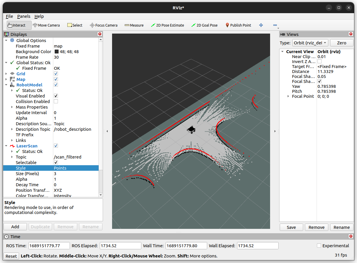
Initializing a node can take a while, so you may need to wait few second until you see generated map. Starting state should be similar to below picture:
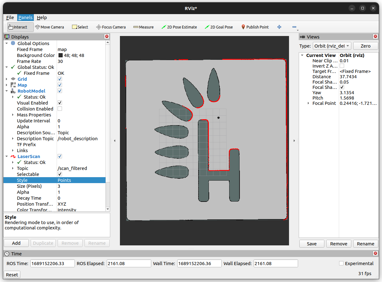
Now drive your robot around and observe as new parts of map are added, continue until all places are explored. Final map should look like below:
Robot mesh visualization does not work if you do not have a locally built and sourced repository with your robot, but this does not affect the robot's behavior.
In this way, a occupancy map was created, where white points indicate free space, black points are a wall or other obstacle, and transparently marked places not yet visited. More about the occupancy map can be found in the next chapter - path planning. Now let's learn how to save the map.
Map
In next example we will use Nav2 packages. Nav2 refers to the Navigation2 package, which is a comprehensive set of software modules for autonomous robot navigation. It is part of the ROS 2 Navigation Stack and is designed to provide advanced navigation capabilities for robots operating in real-world environments. It will be used Nav2 in next amcl chapter. Let's install necessary package:
sudo apt install ros-$ROS_DISTRO-navigation2
sudo apt install ros-$ROS_DISTRO-nav2-bringup
Saving the map
The /map topic is available till node is running, when you close your node you will lose all your explored map. To deal with this you can save map using nav2_map_server package. Save map executing below command and move output to tutorial_pkg/maps.
ros2 run nav2_map_server map_saver_cli -f map
Nav2 create two files (map.yaml & map.pgm) to represent map.
tutorial_pkg/
  └── maps/
    ├── map.pgm
    └── map.yaml
Load saved map
To load the map, you can use the map_server node with the yaml_filename parameter, where you need to specify the stored map. Run map_server inside the maps folder:
- ROSbot
- Gazebo simulator
ros2 run nav2_map_server map_server --ros-args -p yaml_filename:=map.yaml
ros2 run nav2_map_server map_server --ros-args -p yaml_filename:=map.yaml -p use_sim_time:=true
To start map_server you need to run one extra node from nav2.
ros2 run nav2_util lifecycle_bringup map_server
Test result in RViz.
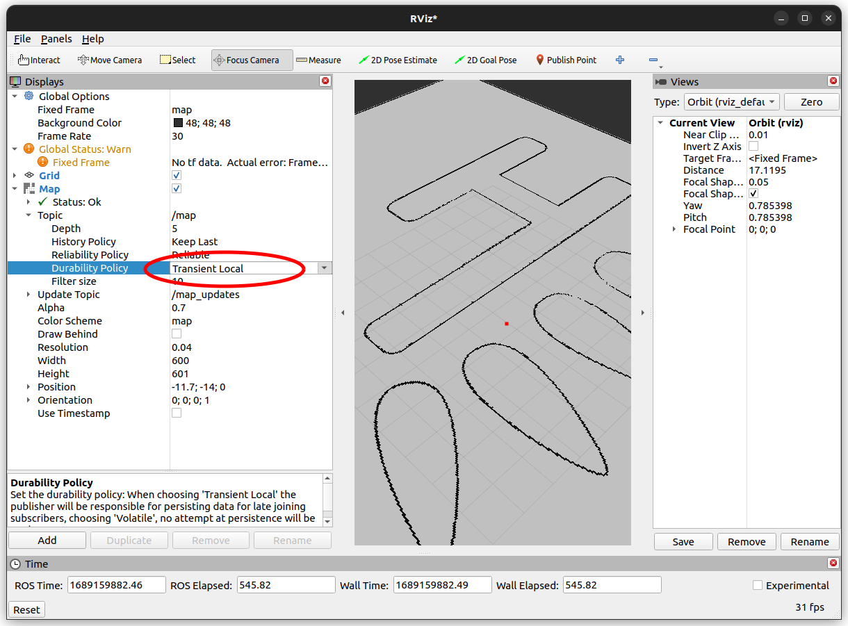
map_server node publish only one msg with map. To display map you have two option:
- Run RViz before running
map_server - Change Map QoS Policy in RViz. Open Map setting and change Topic->Durability Policy to Transient Local.
Localize robot
AMCL is a probabilistic 2D moving robot location system. It implements an adaptive (or KLD sampling) Monte Carlo location approach (described by Dieter Fox) that uses a particle filter to track the position of the robot on a known map.
Basically amcl is no longer a SLAM algorithm because it does not map the environment. However, the principle of operation of the locator can be helpful to better understand the SLAM group of algorithms. For the algorithm to work properly, it must have access to the map and odometry data. With this data, the algorithm of each iteration compares the appearance of the map, along with the current laser scans, and selects only those locations that best match the collected data with the map.
AMCL configuration
As in the case of the slam_toolbox package, amcl also has a lot of parameters necessary for proper operation. Among the most important are:
alphaX- a series of parameters to better match the location depending on the accuracy of the odometrybase_frame_id- name of frame related with robot, in our case it will bebase_link,global_frame_id- name of frame related with map starting point, in our case it will bemap,scan_topic- name of topic with sensor data, in our case it will be/scan_filtered,max_particles- maximum allowed number of particles, in our case it will be set to1000,min_particles- minimum allowed number of particles, in our case it will be set to100,laser_max_range- the maximum usable range of the laser, in our case it will be12.0meters
Again, it is recommended to put all parameters in one amcl.yaml file.
amcl:
  ros__parameters:
    use_sim_time: True
    alpha1: 0.2
    alpha2: 0.2
    alpha3: 0.2
    alpha4: 0.2
    alpha5: 0.2
    base_frame_id: "base_link"
    beam_skip_distance: 0.5
    beam_skip_error_threshold: 0.9
    beam_skip_threshold: 0.3
    do_beamskip: false
    global_frame_id: "map"
    lambda_short: 0.1
    laser_likelihood_max_dist: 2.0
    laser_max_range: 12.0
    laser_min_range: -1.0
    laser_model_type: "likelihood_field"
    max_beams: 60
    max_particles: 500
    min_particles: 50
    odom_frame_id: "odom"
    pf_err: 0.05
    pf_z: 0.99
    recovery_alpha_fast: 0.0
    recovery_alpha_slow: 0.0
    resample_interval: 1
    robot_model_type: "nav2_amcl::DifferentialMotionModel"
    save_pose_rate: 0.5
    sigma_hit: 0.2
    tf_broadcast: true
    transform_tolerance: 1.0
    update_min_a: 0.3
    update_min_d: 0.2
    z_hit: 0.5
    z_max: 0.05
    z_rand: 0.5
    z_short: 0.05
    scan_topic: scan_filtered
    map_topic: map
    set_initial_pose: true
    always_reset_initial_pose: true
    first_map_only: false
    initial_pose:
      x: 0.0
      y: 0.0
      z: 0.0
      yaw: 0.0
You can find detailed explanation of this parameters on official Nav2 documentation
Launch amcl
To run amcl you need to load map with map_server and run amcl node. All nodes in the Nav2 package are only initialized at startup, you need to use lifecycle_manager to run them. Using lifecycle_manager, Nav2 provides a unified way to manage the lifecycle of navigation-related components, making it easier to deploy and control your navigation system in a consistent and reliable manner.
from launch import LaunchDescription
from launch.actions import DeclareLaunchArgument
from launch.substitutions import LaunchConfiguration, PathJoinSubstitution
from launch_ros.actions import Node
from launch_ros.substitutions import FindPackageShare


def generate_launch_description():
    use_sim_time = LaunchConfiguration("use_sim_time")
    amcl_params_file = LaunchConfiguration("amcl_params_file")
    map_file = LaunchConfiguration("map_file")

    use_sim_time_arg = DeclareLaunchArgument(
        "use_sim_time", default_value="false", description="Use simulation/Gazebo clock"
    )

    map_file_arg = DeclareLaunchArgument(
        "map_file",
        default_value=PathJoinSubstitution([FindPackageShare("tutorial_pkg"), "maps", "map.yaml"]),
        description="Full path to the yaml map file",
    )

    amcl_params_file_arg = DeclareLaunchArgument(
        "amcl_params_file",
        default_value=PathJoinSubstitution(
            [FindPackageShare("tutorial_pkg"), "config", "amcl.yaml"]
        ),
        description="Full path to the ROS2 parameters file to use for the amcl node",
    )

    map_server_node = Node(
        package="nav2_map_server",
        executable="map_server",
        name="map_server",
        parameters=[{"use_sim_time": use_sim_time, "yaml_filename": map_file}],
    )

    amcl_node = Node(
        package="nav2_amcl",
        executable="amcl",
        name="amcl",
        parameters=[amcl_params_file, {"use_sim_time": use_sim_time}],
    )

    nav_manager = Node(
        package="nav2_lifecycle_manager",
        executable="lifecycle_manager",
        name="nav_manager",
        parameters=[
            {"use_sim_time": use_sim_time},
            {"autostart": True},
            {"node_names": ["map_server", "amcl"]},
        ],
    )

    return LaunchDescription(
        [
            use_sim_time_arg,
            amcl_params_file_arg,
            map_file_arg,
            map_server_node,
            amcl_node,
            nav_manager,
        ]
    )
To run amcl example type:
- ROSbot
- Gazebo simulator
ros2 launch tutorial_pkg amcl.launch.py
ros2 launch tutorial_pkg amcl.launch.py use_sim_time:=true
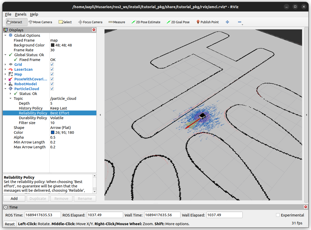
Run RViz on your private computer for visualization. If you don't know how to do it, check the RViz Visualization.
In order for amcl to start working, it needs to be given 2D Estimate Pose corresponding to the real position of the robot. You can now control the robot and watch the program run (you can control it with the teleop_twist_keyboard node). You should get a result similar to the image below, where the purple ellipse under the robot is the position uncertainty and the yellow triangle is the orientation uncertainty. Blue arrows represent potential points where the robot may be.
Task 1 - Inaccurate Initial Pose
In order to better understand the principle of operation of amcl, it is good to give an inaccurate position of the robot. To do this, you can use the 2D Estimate Pose tool in RViz, and then select a point about 1-2m away from the actual position of the robot (default grid size is 1m). The algorithm will automatically improve the position quality after driving a few meters. Remember to observe the actual robot, not the result in RViz, because the position estimation is now bogus - the robot is in a different position than in RViz.
Result and explanation
Below is a graphic that should help you better understand the issues. Description:
- The ROSbot is in a different position than the bet is the computer.
- Arrows represent potential points where the robot may be.
- The best points are selected and new ones are generated near them.
Summary
After completing this tutorial, the concept of SLAM should no longer be foreign to you. From now on, you should know how to run rpLidar and know how to create a map, save it, and fix a location using slam_toolbox. Moreover, you should know how to change the slam_toolbox, map_server and amcl parameters. That's all for now and see you in the next tutorial! 😁
Since the creation of these tutorials, improvements have been made to enhance navigation quality. You can find the latest demos for our robots at the following links:
by Rafał Górecki, Husarion
Need help with this article or experiencing issues with software or hardware? 🤔
- Feel free to share your thoughts and questions on our Community Forum. 💬
- To contact service support, please use our dedicated Issue Form. 📝
- Alternatively, you can also contact our support team directly at: support@husarion.com. 📧